Posture and Horns!
Introduction
This project focuse on this article published by Nature Scientific Reports. The original research describes the relationship between posture and “enlarged protuberances”, especially among younger subjects. This was later reported in the popular press in articles drawing the conclusion that phone usage was leading to “horns” growing in the back of millenials’ heads. Later articles were more skeptical, and a limited author correction was published in Nature.
The goals of the project is to revisit the data that has been used in this research (data that accompanied the author correction), and do the following:
Look at some distributions of subjects
Illustrate issues in the available data
Redo the flawed analysis in the research paper
Adding some visualization that helps answering the scientific question of interest
Reproducing reported results and find possible inconsistensies
Discussing the findings
Data Cleaning
eop_data = read_excel("mtp_data/p8105_mtp_data.xlsx", skip = 7) %>%
  janitor::clean_names() %>%
  select(sex, age_group, age, eop_size_group = eop_size, eop_size = eop_size_mm,
         eop_visibility_class = eop_visibility_classification, eop_shape,
         fhp_category, fhp_size = fhp_size_mm) %>%
  filter(age_group > 1) %>%
  mutate(
    eop_size = replace_na(eop_size, 0),
    sex = factor(sex),
    eop_visibility_class = factor(eop_visibility_class, levels = c('0', '1', '2'), ordered = TRUE),
    eop_shape = factor(eop_shape, levels = c(1, 2, 3)),
    age_group = factor(age_group, levels = c('2', '3', '4', '5', '6', '7', '8'),
                       labels = c('18-30', '31-40', '41-50', '51-60', '60+',
                                  '60+', '60+'), ordered = TRUE),
    eop_size_group = factor(eop_size_group, levels = c('0', '1', '2', '3', '4', '5'),ordered = TRUE),
    fhp_category = factor(fhp_category, levels = c('0', '1', '2', '3', '4', '5', '6', '7'), ordered = TRUE)
  )
Resulting dataset has 9 variables of 1219 participants, with key variables age(age_group), sex, fhp_category, and eop_size(eop_size_category).There were 613 women and 606 men. Sex distribution across age_groups:
  age_sex_table = eop_data %>%
   group_by(age_group, sex) %>%
   summarize(count = n()) %>%
   pivot_wider(
     names_from = age_group,
     values_from = count
   ) %>%
   mutate(sex = recode(sex, `0` = "Female", `1` = "Male")) %>%
knitr::kable()| sex | 18-30 | 31-40 | 41-50 | 51-60 | 60+ |
|---|---|---|---|---|---|
| Female | 151 | 102 | 106 | 99 | 155 |
| Male | 152 | 102 | 101 | 101 | 150 |
Data Issues
cat_eop = eop_data %>%
  group_by(eop_size, eop_size_group, eop_visibility_class) %>%
  filter(eop_size == 5 | eop_size == 10 | eop_size == 15 | eop_size == 20 | eop_size == 25) %>%
  summarize(count = n()) %>%
  knitr::kable()
2 people aged 17 and 45 in age_group=1 which had not been defined. Participants age range=18, 88(reported:18,86). Table shows overlaps in continuous-categorical coversion. In eop_category cut-offs: Same eop_size(5) is associated with different size_categories(0,1) and visibility_groups(1,2). One mistaken eop size group(14.6) noted (shows as ‘NA’ since not among defined factor levels). We should have 8 FHP categories(0-7) but we have9,because of mistaken value(30.8).
| eop_size | eop_size_group | eop_visibility_class | count |
|---|---|---|---|
| 5 | 0 | 2 | 1 |
| 5 | 1 | 1 | 1 |
| 5 | 1 | 2 | 2 |
| 10 | 2 | 2 | 1 |
| 15 | 3 | 2 | 2 |
| 15 | NA | 2 | 1 |
| 20 | 3 | 2 | 2 |
Also, 8 people with eop_visibility_class=1, but eop_size>5.
73 with eop_size=0 but eop_visibility_class other than 0.
1 with eop_size=11.3 but eop_visibility_class=0.
5 with eop_size<5 but eop_visibility_class=2.
Visualization
In the original scientific report, Figures 3 and 4 show data or derived quantities. Both are flawed. Figure 3 shows only the mean and standard deviation for FHP, but does not show the distribution of the underlying data. Figure 4 shows the number of participants in each age and sex group who have an enlarged EOP (based on categorical EOP Size – groups 0 and 1 vs groups 2, 3, 4, and 5). However, the number of participants in each age and sex group was controlled by the researchers, so the number with enlarged EOP in each group is not as informative as the rate of enlarged EOP in each group. I Created a two-panel figure that contains improved versions of both of these:
# Boxplot for fhp distribution
fhp_age_dist = eop_data %>%
  ggplot(aes(x = age_group, y = fhp_size)) +
  geom_boxplot(aes(fill = sex)) +
  labs(
    title = "FHP Distribution Across Age Group",
    x = "Age Groups (years)",
    y = "FHP Size (mm)",
    caption = "Figure 3 modified to show distribution instead of mean and median"
  ) +
  scale_fill_discrete(name = "Sex", labels = c("Female", "Male")) +
  theme(
    legend.position = c(.5, .95),
    legend.justification = c("right", "top")
    )

# EEOP rate plot
eeop_rate_plot = eop_data %>%
  group_by(age_group, sex) %>%
  mutate(group_n = n()) %>%
  group_by(age_group, sex, group_n) %>%
  filter (
    eop_size_group > 1
  ) %>%
  summarize(eeop_n = n()) %>%
  mutate(
    rate = eeop_n /group_n
  ) %>%
    ggplot(aes(x = age_group, y = rate, color = sex, group = sex)) +
  geom_point() +
  geom_line() +
    labs(
    title = "Rate of EEOP Across Age Groups",
    x = "Age Groups (years)",
    y = "EEOP Rate",
    caption = "Figure 4 modified to show rate of EEOP instead of count"
  ) +
  scale_colour_discrete(name = "Sex", labels = c("Female", "Male")) +
  theme(
    legend.position = c(.5, .95),
    legend.justification = c("right", "top")
    )

# joining plots using patchwork
(fhp_age_dist + eeop_rate_plot)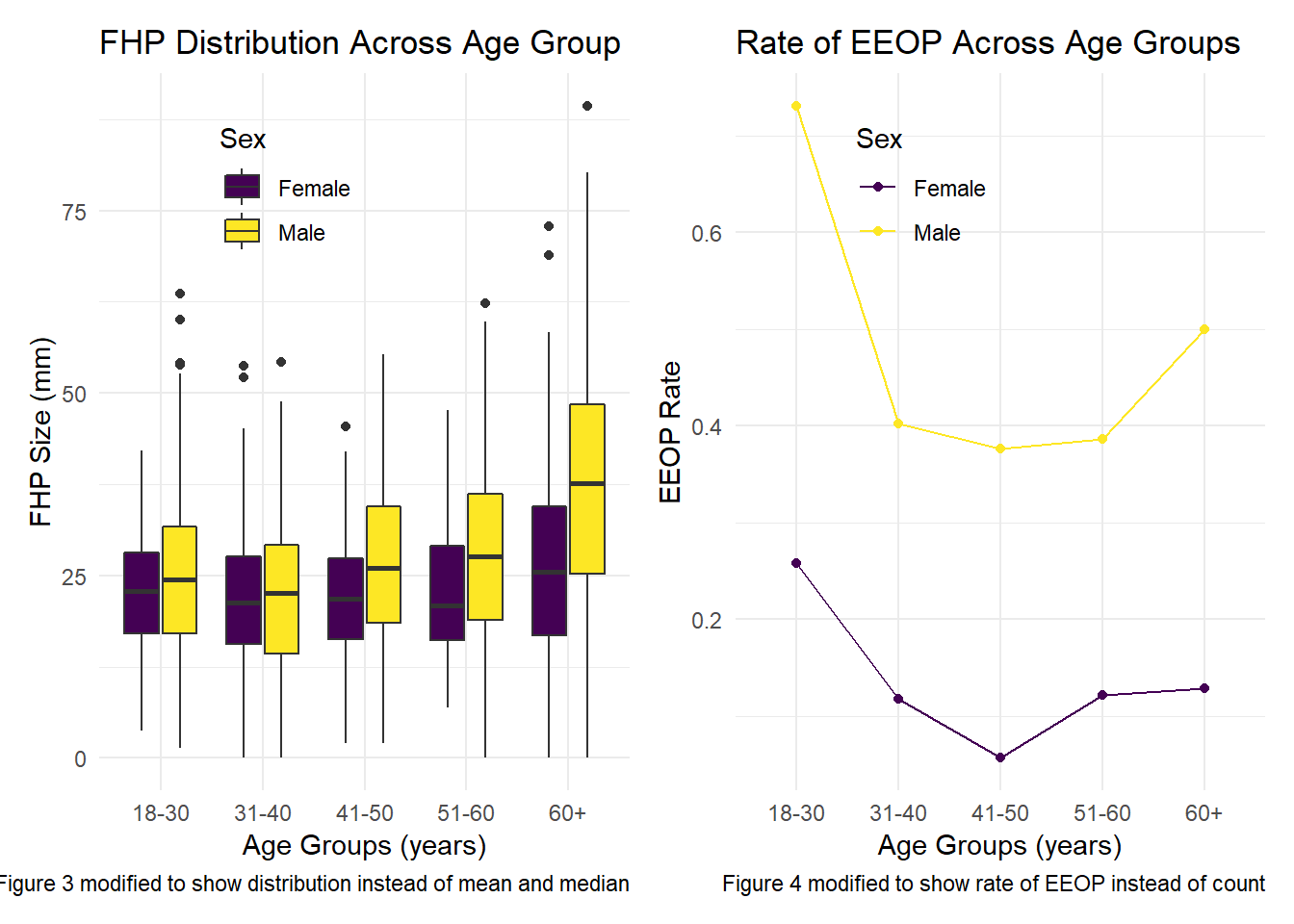
In higher age_groups fhp_size is more spread (higher IQR), and increased in median value by sex mostly. Also, increased difference of median fhp_size between men and women. Higher FHP_size median and IQR for men and in age60+. We cannot see as strong effect on other groups.
There is high eeop_rate among 18-30, but plots get flatter after that(compared to count plot). This shows that there is higher chance of eeop in this group compared to others, cannot generalize about other groups.
Although the authors are interested in how FHP size, age, and sex affect EOP size, no figure contains each of these in the research paper. I created a 2 x 5 collection of panels, which shows the association between FHP size and EOP size in each age and sex group:
collection_plot = eop_data %>%
  ggplot(aes(x = fhp_size, y = eop_size, color = sex)) +
  geom_point() +
  facet_grid(sex ~ age_group,
             labeller = labeller(sex = as_labeller(c("0" = "Female", "1" = "Male")))) +
  labs(
    title = "Effect of key Variables on EOP Size",
    x = "FHP Size (mm)",
    y = "EOP Size (mm)",
    caption = "This 2x5 plot shows the distribution of EOP_size vs. FHP_size, in men and women and
    across different age_groups"
  ) +
  theme(legend.position = "None")

collection_plot 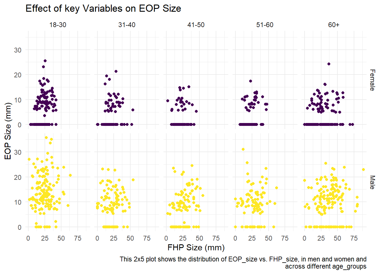
Generally, we can observe dispersed distribution(most disperesed in men 18-31 and 60+), and there is no specific trend for how eop_size changes with increase of FHP_size in different groups. With performing complementary statistical tests, we might conclude there is no association between these variables. However, according to the article, increase in fhp_size is linked to increase in eop_size.
Reproducing Reported Results
In this part, I tried to see…
If the authors’ stated sample sizes in each age group consistent with the data available
I the reported mean and standard deviations for FHP size consistent with the data you have available?
The authors find “the prevalence of EEOP to be 33% of the study population”. Is the finding consistent with the data available?
FHP is noted to be more common in older subjects, with “FHP >40 mm observed frequently (34.5%) in the over 60s cases”. Are the broad trends and specific values consistent with data?
sample_size = eop_data %>%
  group_by(age_group) %>%
  summarize(sample_size = n()) %>%
  mutate(
    reported_sample_size = c("300", "200", "200", "200", "300")
  ) %>%
  knitr::kable()


eeop_prevalence = eop_data %>%
  filter(eop_size > 10) %>%
  nrow()/nrow(eop_data)

sixties_n = eop_data %>%
  filter(age > 60) %>%
  nrow()

fhp_n = eop_data %>%
  filter(age > 60 & fhp_size > 40) %>%
nrow()| age_group | sample_size | reported_sample_size |
|---|---|---|
| 18-30 | 303 | 300 |
| 31-40 | 204 | 200 |
| 41-50 | 207 | 200 |
| 51-60 | 200 | 200 |
| 60+ | 305 | 300 |
Table above shows that sample size for each age_group does not match reported figures. Also data contains a “group 1”(n=2) for age 17,45, which is not reported.
Repored mean FHP_size is “26 ±mm”. The value of standard deviation is not clear. The true FHP size mean for this sample is 26.08 ±13.01mm. This is high deviation and should have noted in statistical inference.
Eop_size>10 is enlarged. Prevalence is number of diseased people in total population. So, number of enlarged EOP people and total participants are needed. Result: 32.2%, different from reported(33%).
There are 305 people in age_group(60+), within which 99 have FHP_size>40(mm): frequency is 32.46%, not 34.5%. Broad trend shows higher FHP in 60+ group(much higher in men), but other age_groups don’t show increasing trend:
high_fhp_plot = eop_data %>%
  filter(fhp_size > 40) %>%
  group_by(age_group, sex, fhp_size) %>%
  summarize(
    n = n()
  ) %>%
  ggplot(aes(x = age_group, fill = sex)) +
  geom_bar(position = 'dodge') +
  labs(
    title = "Number of cases With Large FHP (FHP Size > 40) Across Age Groups",
    x = "Age Groups (years)",
    y = "Number of cases",
    caption = "Plot shows that the broad trend on high FHP size with age is high in 60+ group
    also, it is always greater in men than women, but there is no other uniform trend in data."
  )

high_fhp_plot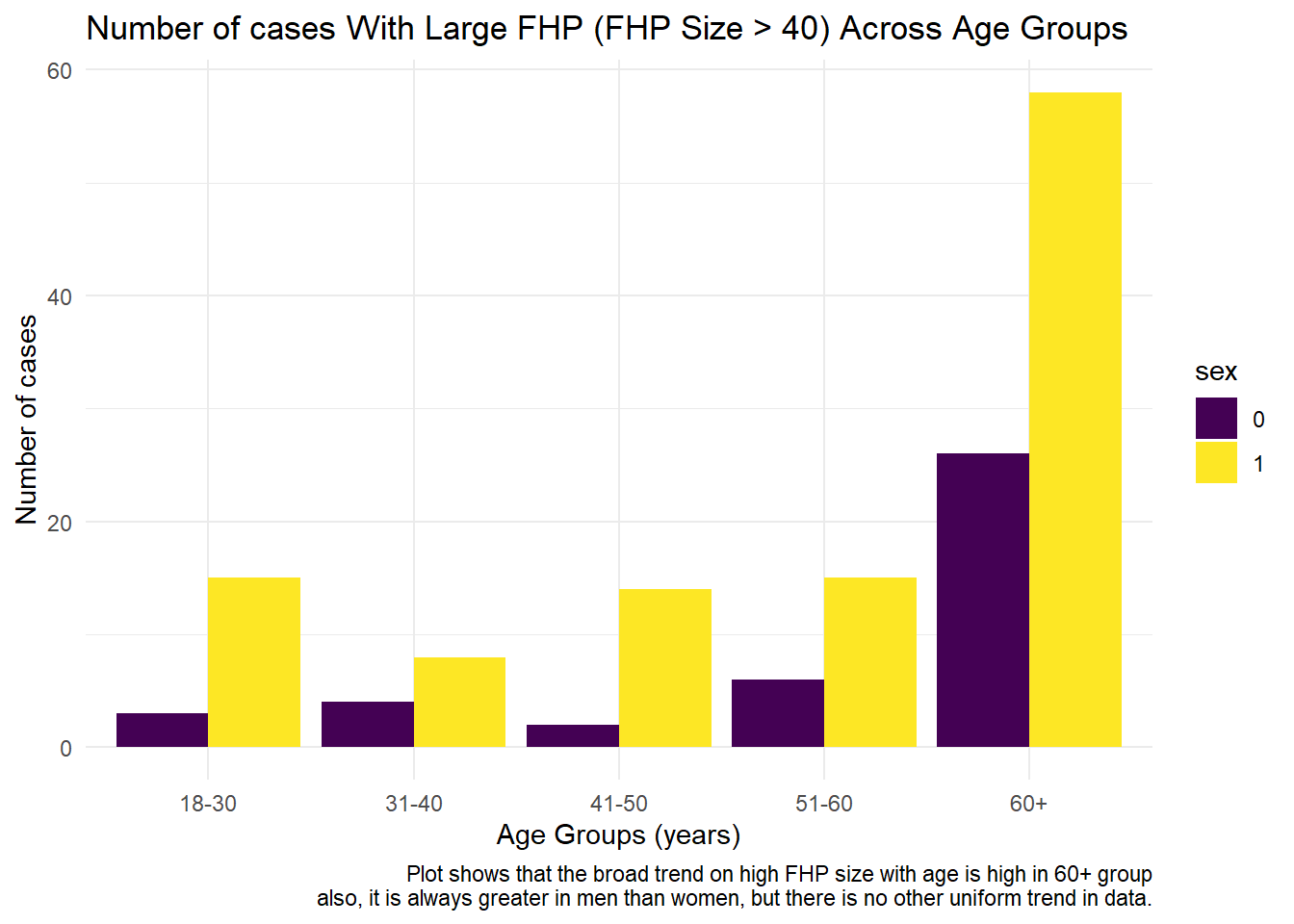
Discussion
Authors conclude high Eop in result of age and fhp combination. However, it is not a general trend in data. Also, 18-30 age group have high eop but there is no evidence where it comes from (another possible explanation can be that young people who were visiting clinic might have genetic problems, have had an accident, etc.). Also, it doesn’t seem that people with higher fhp tend to have higher eop. Statistical analysis of research only relies on P-value which is not reliable without Confidence intervals. Analysis and sample size were not reported accurately and have been rounded, and in general, plots seem to be cherry-picked to justify the desired result. Source population were more prone to outcome (people visited clinic): Conslusions are only generalizable to the cohort and not to general population.
Other data is needed to address this hypothesis. For example, data on the reson that patients visited clinic is needed. Also, we need to have data on the approximate time people spent on electric devices and cellphone are needed. It is also important to know their occupation, their physical activity and diet which affects skeletal health. Also, researchers should have controlled study for genetic variability(race/ethnicity). Results say nothing about causal link between cell-phone and horn growth! Can just discuss “possible” association between poor posture and EEOP, if all required information provided and controlled for confounders.